Microsoft Excel is a spreadsheet application written and distributed by Microsoft for Microsoft Windows and Mac OS X. Microsoft Excel has the basic features of all spreadsheets, using a grid of cells arranged in numbered rows and letter-named columns to organize data manipulations like arithmetic operations. It basically depends on our knowledge about its various formulae and functions and hence it is very powerful when compared with others. It is useful for many applications.
It is very user friendly as a whole; it is generally have click application for easy handling. There are many more unknown features of it to others. So you have to explore it for additional useful information. The following steps help us in hiding the cell contents of Excel collectiveRay.com.
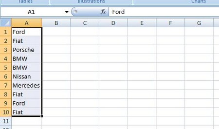
Start Microsoft Office and choose Microsoft Excel. If any workbook already exists then open any existing workbook that contains cells you would like to hide the contents. If there is no workbook then start a new workbook.
To create a fresh one, just go to the menu at the top of Excel home page. Then go to new command and click it. Once you click new command, a new workbook page will open. Then you can enter some content into a cell which you would like to hide.
If you need to make your cells bigger in Google sheets or excel, you can simplify it but merging certain cells together and making them one bigger cell. This is a great way to add more content to one large cell and not having them overlap onto one another. If you would like to know how to accomplish this, there is a simple tutorial here on merging cells in sheets that can help you complete this task.
There may be several cells with its data. Sometime we want to hide all the contents. But sometime, we want to hide only selective contents of the cell. If you want to hide all the contents, then select all the cells.
If you want to hide only selective contents then select the cells that contain data you would like to hide. You can select cells by clicking on them and using the SHIFT or CTRL keys on your keyboard to select additional cells.
The next step after choosing the cells to hide is to format the contents. To do those choose the “Format” from menu and click “Cells”. Then it will open the “Format Cells” dialog box.
Next click on the “Number” tab in the “Format Cells” dialog box. It is to display the formats that can be applied to Excel cells as there are a number of different formats. There are many inbuilt formats; if we want to have your own formats then you can do that using the custom settings.
It helps us to create your own format which you want to apply. Select “Custom” from the “Category” text box so you can type your own custom formatting to hide your selected cells.
Type 3 semicolons (;;;) in the “Type” text box to tell Excel that you want to hide the cells. Click the “OK” button to close the “Format Cells” dialog box and hide the selected cells.
